2. Economic dispatch as a linear optimisation problem

2.1. Economic dispatch

We start by looking at a simple problem. We are a power company that owns two power plants. We know what demand for power is going to be in the next hour, and we need to decide how to operate our power plants to meet that demand while minimising our cost. To do so we decide which of our plants should be operating, and if they are operating, how much electricity they should be generating. The problem is illustrated in Fig. 2.1.

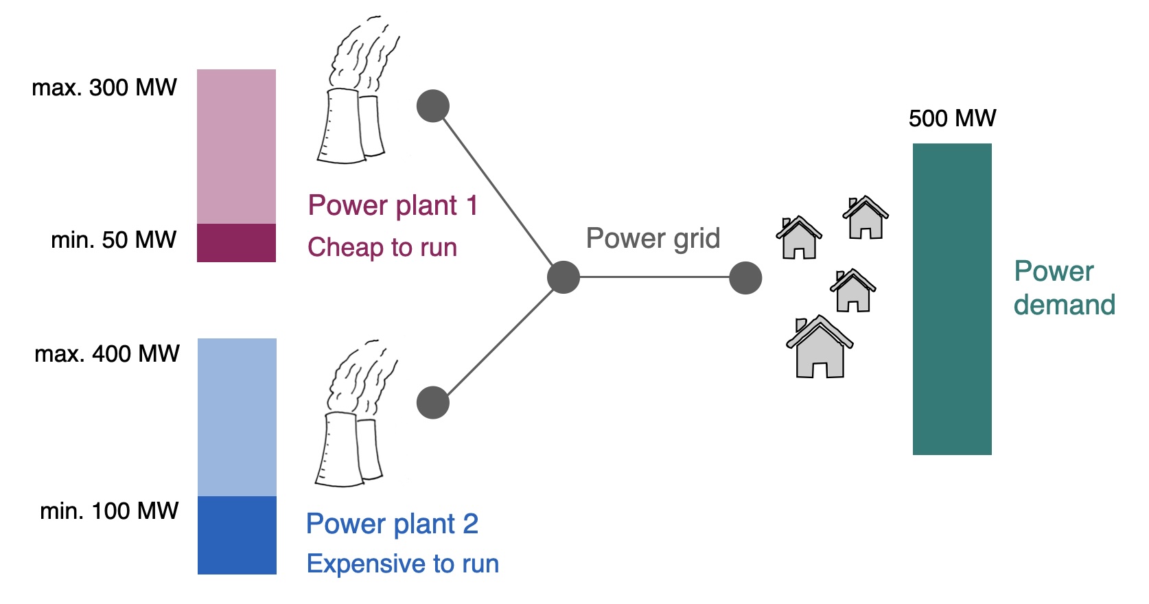
Fig. 2.1 An illustrative economic dispatch problem with two power plants.

We call this the economic dispatch (ED) problem. More generally, the problem is to distribute the total power demand among available power generators (also called “units” or “generating units”) in a way that minimises the total power generation cost. Each generating unit has different power generation costs based on how it generates power. What we usually consider in this kind of problem is the marginal cost, so, the cost of providing one additional unit of electricity. This implies that we do not consider the cost of building the power plant, only of operating it now that it exists.

For a thermal power plant, for example, the main contributor to the power cost is the cost of fuel. These costs can vary significantly across different units, for instance, the power generation costs for a nuclear unit and a gas-fired unit will differ widely. In addition, renewable generators like a wind farm have no or very small marginal generation costs, since their main resource - wind in the case of a wind farm - is free. We will return to that issue later.

A note on terminology

In the context of “economic dispatch”, you will frequently hear these terms:

• Unit commitment: This is a more general problem that we will return to later, which includes additional considerations, for example the fact that power plants can be turned on and off (but they might require time, or additional costs, to do so). Economic dispatch can be considered a sub-problem of unit commitment.

• Merit order: You will also hear “merit order” in the context of dispatch. This simply refers to the approach of ranking different generating units or sources of electricity based on their “merit”. If we consider only costs, then the merit order is the solution to the economic dispatch problem.

2.2. Mathematical optimisation

To formulate a mathematical optimisation problem, we will generally need four components.

First, we have some 0 parameters, known quantities that remain fixed. Second, we have the 1 decision variables, the quantities we do not know and would like to find optimal values for.

In order to find optimal values for the variables, we need to know what we are looking for. That is where the 2 objective function comes in: this is a function made up of our variables that we seek to either minimise or maximise. For example, if we want to minimise cost across all our power plants, our objective function would represent that cost by summing up each individual plant’s cost.

Finally, we likely have some 3 constraints. These are expressions that limit the values that our variables can take. For example, if we have a variable describing the power generation of a power plant, we would want to constrain that variable so that its maximum value is the rated power output of the power plant.

In summary, these are the four components of an optimisation problem - we will use this structure whenever we think through a problem formulation:

• 0 Parameters

• 1 Variables

• 2 Objective

• 3 Constraints

2.3. Economic dispatch as an optimisation problem

Now that we’ve introduced economic dispatch (Section 2.1) and the basic concept of optimisation (Section 2.2), we can formulate the economic dispatch problem from Fig. 2.1 as a linear optimisation problem. “Linear optimisation” means that both our objective function and all of the constraints are linear, continuous functions.

We assume that we’re looking at a one-hour time frame and ignore everything that happens before and after that hour.

“Programming” in the context of optimisation

Linear optimisation is often called “linear programming” and abbreviated to LP. “Programming” in this context does not mean “computer programming” in the modern sense but comes from the history of how these methods were developed in the United States during World War II, where “programming” referred to logistics scheduling in the military. We will use “programming” and “optimisation” interchangeably.

2.3.1. 0 Parameters

We know the demand for the hour we are looking at, \(P_{demand}\) = 500 MW.

We also know some things about our power plants (units). We know what their minimum and maximum power generation are. We will call that \(P_{min,i}\) and \(P_{max,i}\), for each unit \(i\).

We also know how much it costs us to run our units for an hour. For now, we will assume that the cost is simply a function of the power output over the hour that we are considering. Thus, our per-unit cost is \(C_i\), representing the unit \(i\)’s generating cost in €/MW.

The specifics of our two units are:

• Unit 1 is a coal-fired power plant: Cost is 3 EUR/MW, minimum output is 50 MW, maximum output 300 MW

• Unit 2 is a gas-fired power plant: Cost is 4 EUR/MW, minimum output 100 MW, and maximum output 400 MW

2.3.2. 1 Variables

We want to decide how to operate our units, so our variables - the unknown quantities that we want to optimise - are the power generated in each unit \(i\):

\(P_i\)

2.3.3. 2 Objective

Our objective is to minimise our cost of generating power. Given the cost per unit, \(C_i\), and the power generated in each unit, \(P_i\), we can formulate the total cost as follows:

(2.1)\[\begin{equation} \label{eq:ed_cost} C = \sum_{i=1}^{n} C_i * P_{i} \end{equation}\]

2.3.4. 3 Constraints

We have two practical constraints to consider.

First, our units must operate within their physical limits - their generated power must be between their minimum and maximum possible output:

(2.2)\[\begin{equation} \label{eq:ed_min} P_{min,i} \leq P_{i} \leq P_{max,i} \end{equation}\]

Second, the amount of electricity generated must exactly match the demand for electricity:

(2.3)\[\begin{equation} \label{eq:ed_balance} \sum_{i=1}^{n} P_{i} = P_{demand} \end{equation}\]

Note this implies that we ignore many practical matters, for example:

• We have perfect knowledge about everything, e.g. we know demand exactly.

• We ignore the fact that demand and supply are separated in space; i.e. there are no grid losses of electricity.

2.3.5. Full problem

In our example, with two power plants, we end up with the following linear optimisation or linear programming (LP) problem:

• Variables: \(P_1\) and \(P_2\)

• Objective (to be minimised): \(C = C_1 * P_1 + C_2 * P_2 = 3P_1 + 4P_2\)

• Demand balance constraint: \(P_1 + P_2 = 500\)

• Operational constraint for unit 1: \(50 \leq P_1 \leq 300\)

• Operational constraint for unit 2: \(100 \leq P_2 \leq 400\)

2.4. Graphical solution

Since this is a two-dimensional problem, with our two decision variables \(P_1\) and \(P_2\), we can visualise the solution graphically. In principle, we are looking for a value for \(P_1\) and \(P_2\), so a point in the two-dimensional decision space seen in Fig. 2.2.

To find the best solution, we first need to identify the feasible region. This region includes all feasible points, that is, points that meet the constraints of the problem.

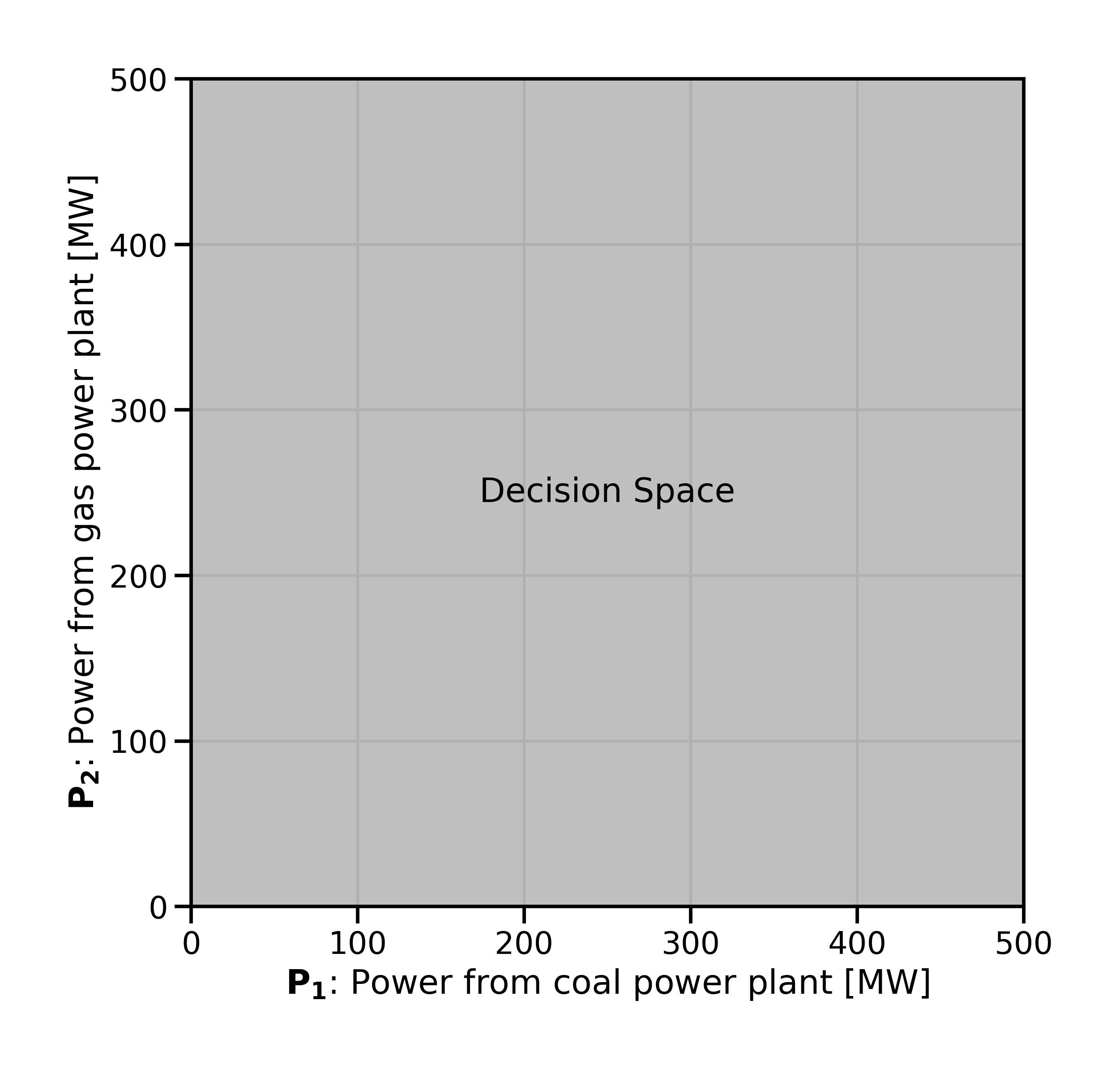
Fig. 2.2 The two-dimensional decision space.

First, we can draw in the operational constraints for both units. These constraints are inequality constraints: they state that a variable must be lesser or equal to, greater than or equal to, a specific value. This gives us a feasible region bounded on all sides, as seen in Fig. 2.3.

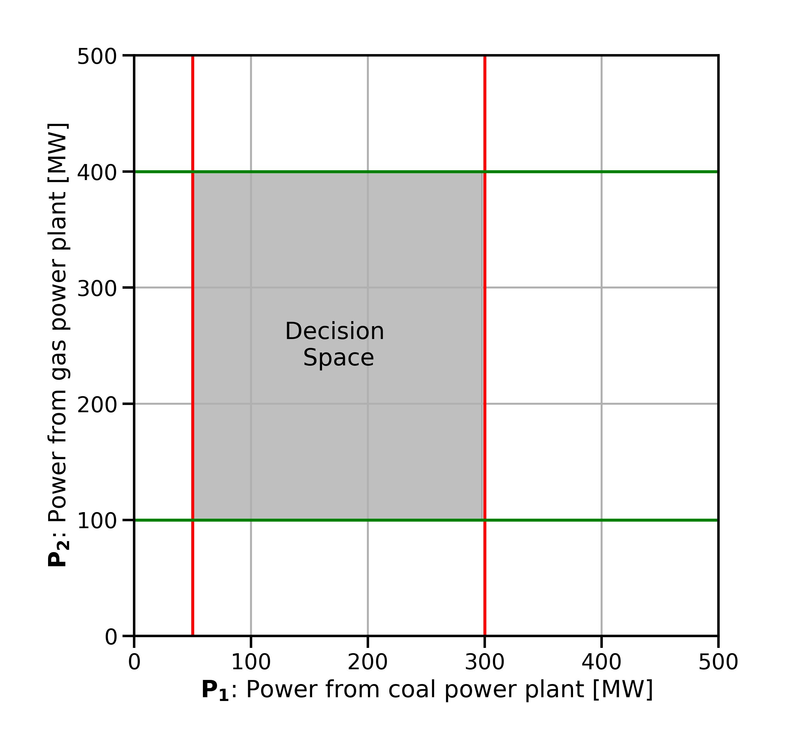
Fig. 2.3 The two-dimensional decision space with the operational constraints for both units shown in red (\(P_1\)) and green (\(P_2\)).

Next, we need to consider the demand constraint. The demand constraint is an equality constraint. We want a linear combination of the supply variables to add up to exactly the known power demand for the hour, 500 MW. In combining the operational constraints from above with the demand constraint, we end up with a feasible region which in this case is just a line segment (Fig. 2.4).

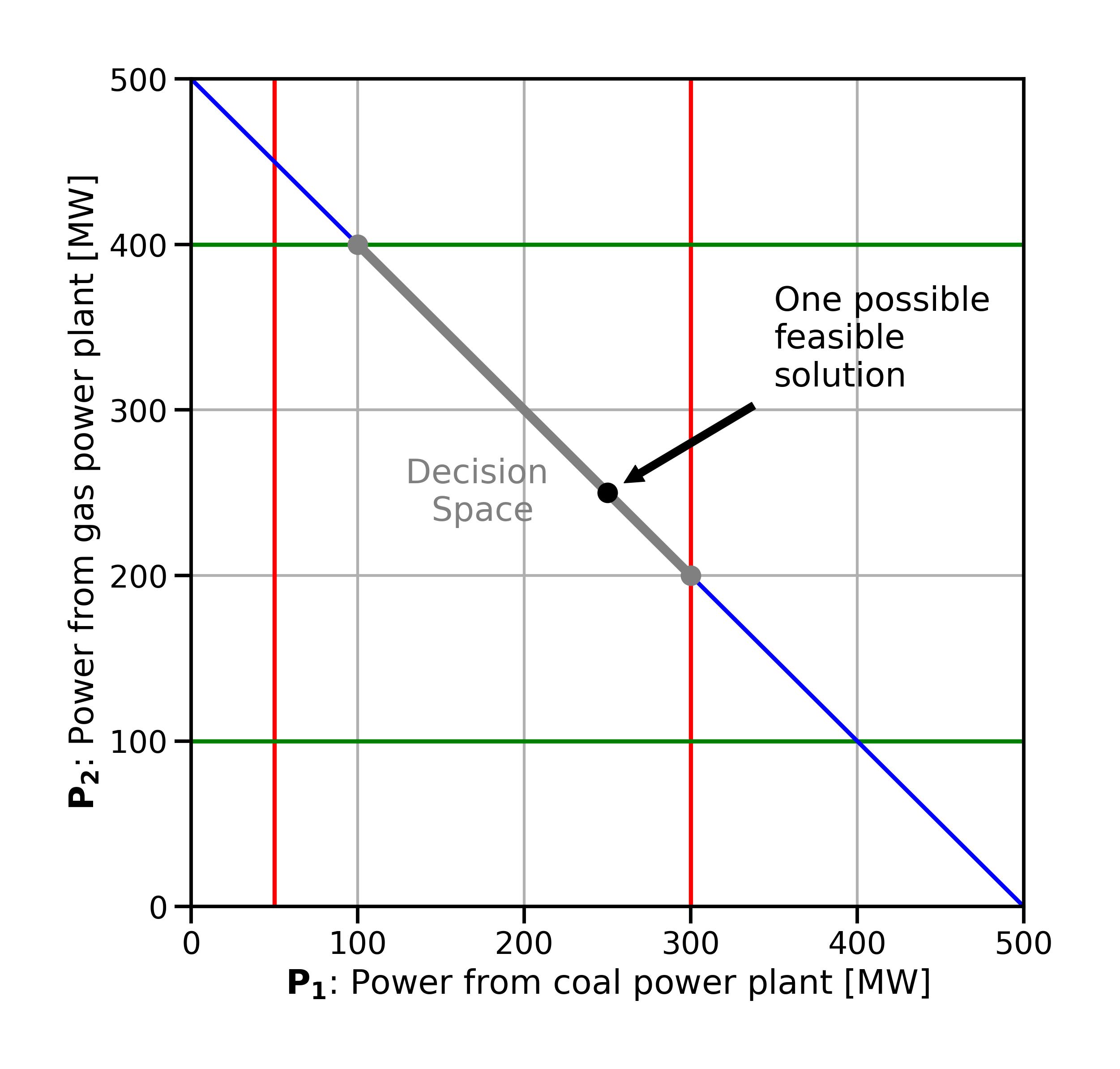
Fig. 2.4 The two-dimensional decision space after the addition of the demand constraint. The feasible region is now a line segment (grey).

The best solution, or optimal solution, is a feasible point that gives the highest or lowest value of the objective function. The corners of the feasible region, where two or more constraints intersect, are the extreme points. An optimal solution, if it exists, will be an extreme point. There may be more than one optimal solution (we will look at such a case below).

If it is impossible to meet all constraints (the problem is infeasible) or the constraints don’t form a closed area (the problem is unbounded), then there is no solution at all.

To find the optimal solution, we can calculate the objective function’s value at each extreme point (Fig. 2.5). The point that gives the best value is the optimal solution. This method is impractical for problems with many variables and constraints but works for problems with just two decision variables.

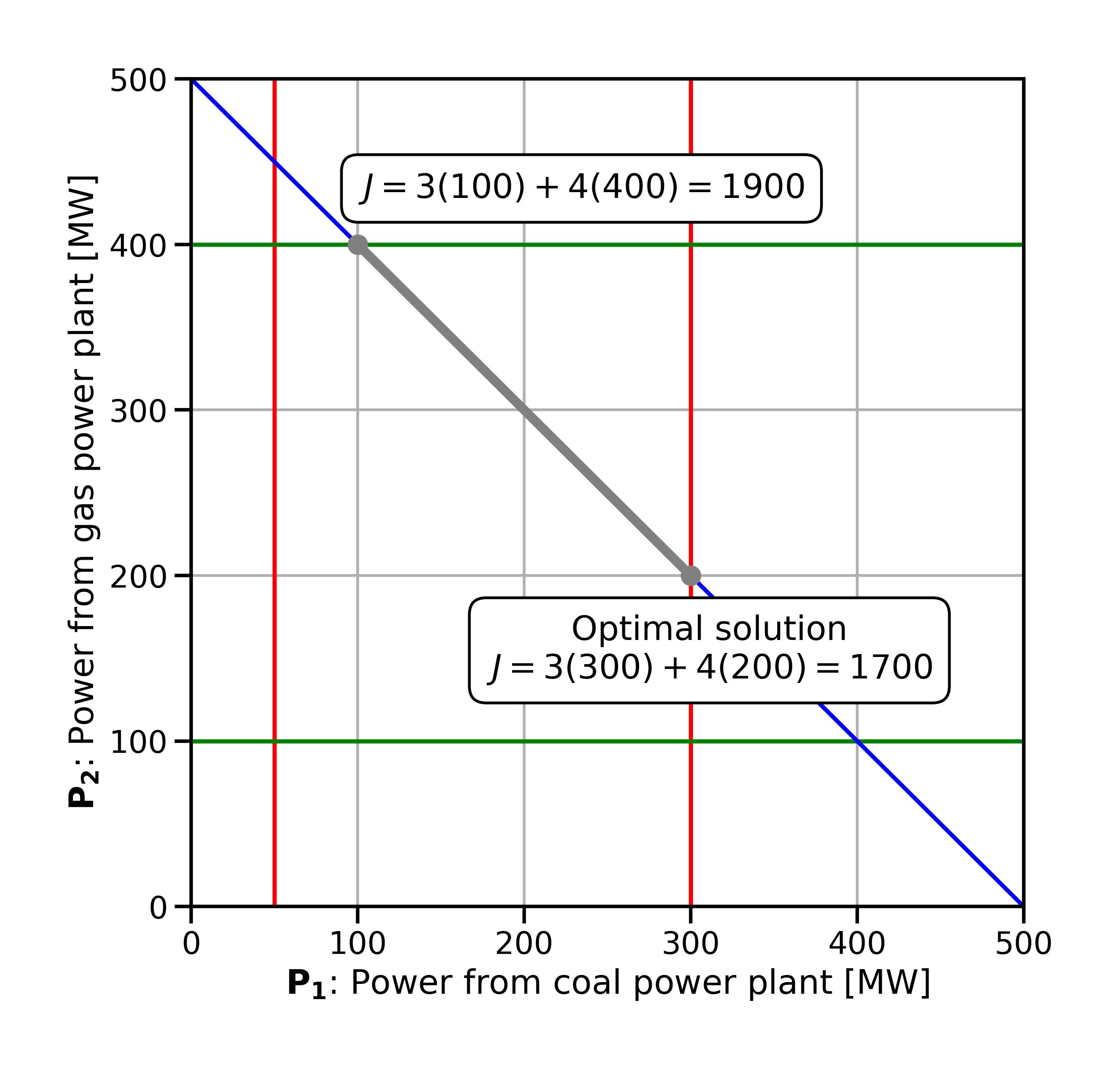
Fig. 2.5 Iteratively looking for the optimal solution by evaluating the objective function value at all of the corners of the feasible space (in this case, there are two “corners” since the feasible space is a line segment).

Why is an optimal solution, if it exists, going to be at one of the extreme points? To understand this, we can use contour lines (also called isolines).

2.5. Contour lines

A contour line is “a curve along which the function has a constant value, so that the curve joins points of equal value” (see Wikipedia, and Fig. 2.6 below). Topographic maps use contour lines to show the shape of the three-dimensional landscape on a two-dimensional paper or screen.

Fig. 2.6 Illustration of contour lines. From Wikipedia (CC-BY 2.5).

Similarly, we can use contour lines to visualise the “third dimension” representing the value of the objective function in our two-dimensional variable space. Because our objective function is linear, the contour lines are straight lines. They represent the projection of the three-dimensional “objective function plane” into the two-dimensional variable space.

To draw contour lines, we set the objective function to a given value (since we already know that 1700 is the optimum, let’s start with that). We can transform the objective function equation into a two-dimensional function. Thus,

(2.4)\[\begin{equation} C = 1700 = 3 P_1 + 4 P_2 \end{equation}\]

becomes

(2.5)\[\begin{equation} P_2 = 425 - 0.75 P_1 \end{equation}\]

To draw further lines we increase and decrease the value by a constant value and repeat the process. In Fig. 2.7 we can see what this looks like. In the direction towards the upper right of the plot, the objective function value decreases, in the direction of the lower left of the plot, it decreases. Looking at teh contour lines, we can imagine that we are walking “downhill” in a direction perpendicular to the parallel contour lines (since we are minimising) inside the feasible space, until we hit the edge of the feasible space and cannot go downhill any further - this is the optimum.

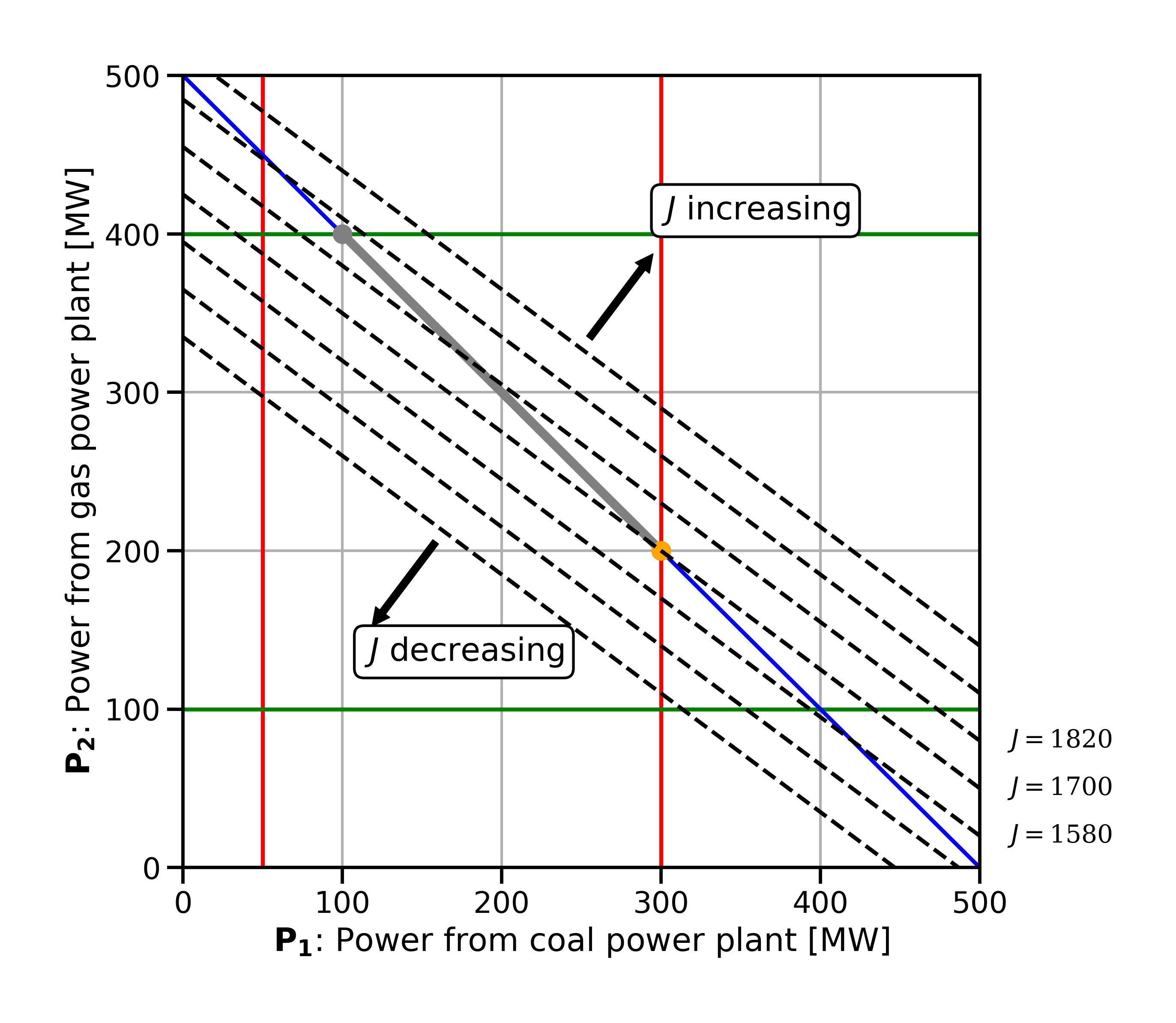
Fig. 2.7 Contour lines of the economic dispatch problem.

What if we change our objective function slightly so that both coefficients are \(4\)? The objective function becomes:

(2.6)\[\begin{equation} C = 4 P_1 + 4 P_2 \end{equation}\]

Drawing the contour lines of this revised objective function, we can see that they are parallel to the feasible space (Fig. 2.8). If we go “downhill” along these lines, we cannot end up in a single point - any point along the contour line overlapping with the feasible space is an equally good solution. This illustrates that depending on how the constraints and objective function are set up, a problem may have not just one but an infinite number of optimal solutions.

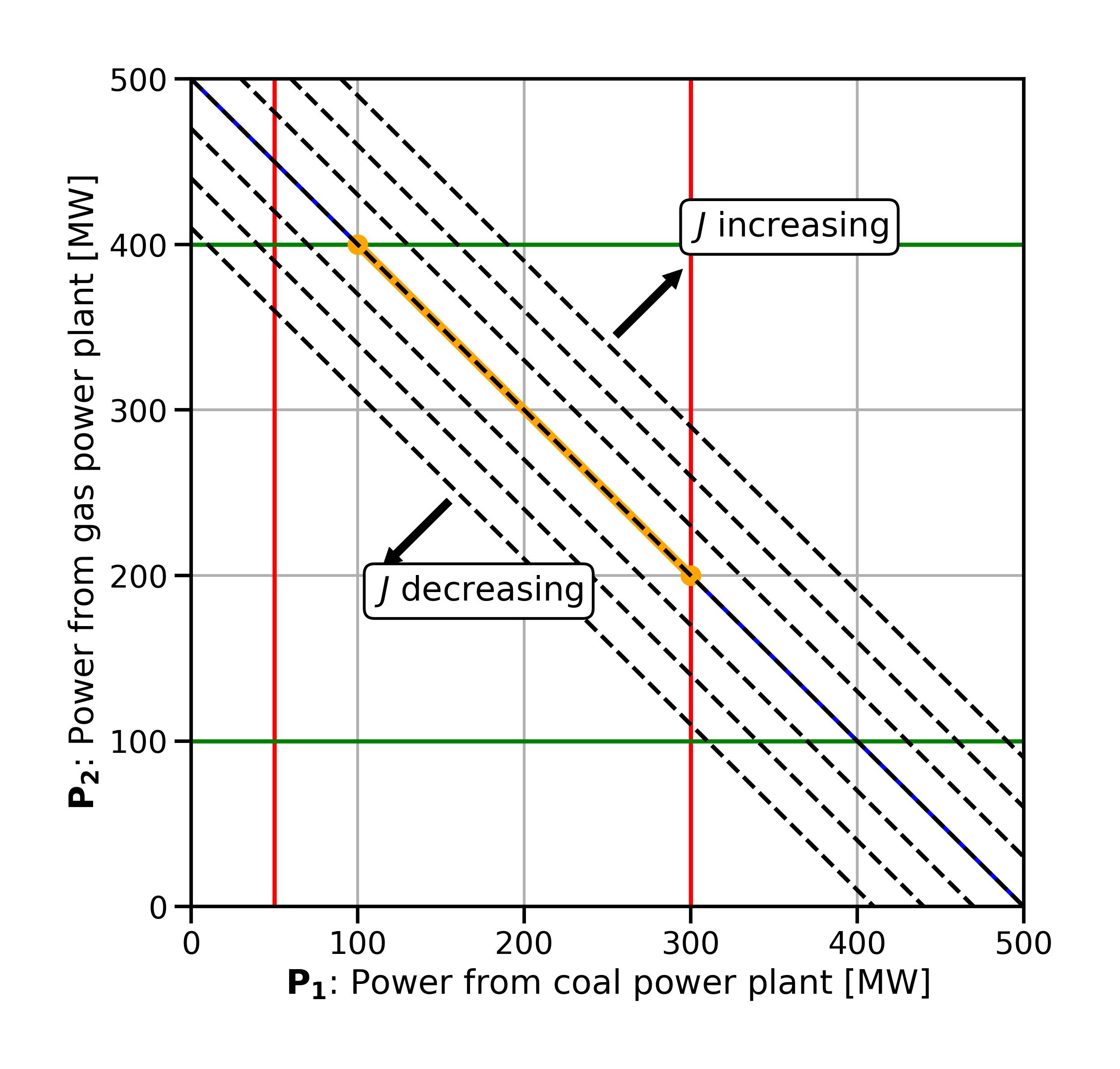
Fig. 2.8 Contour lines of the economic dispatch problem with revised objective function.

2.6. Active constraints

Finally, let’s look at the active constraints. These are the constraints that “force” the objective function to the value it takes in the optimum. In other words, they are the binding constraints. In our example, two constraints are active / binding (see Fig. 2.9):

• the maximum output constraint for \(P_1\): \(P_1 <= 300\)

• the demand constraint (note that by definition, equality constraints are always active)

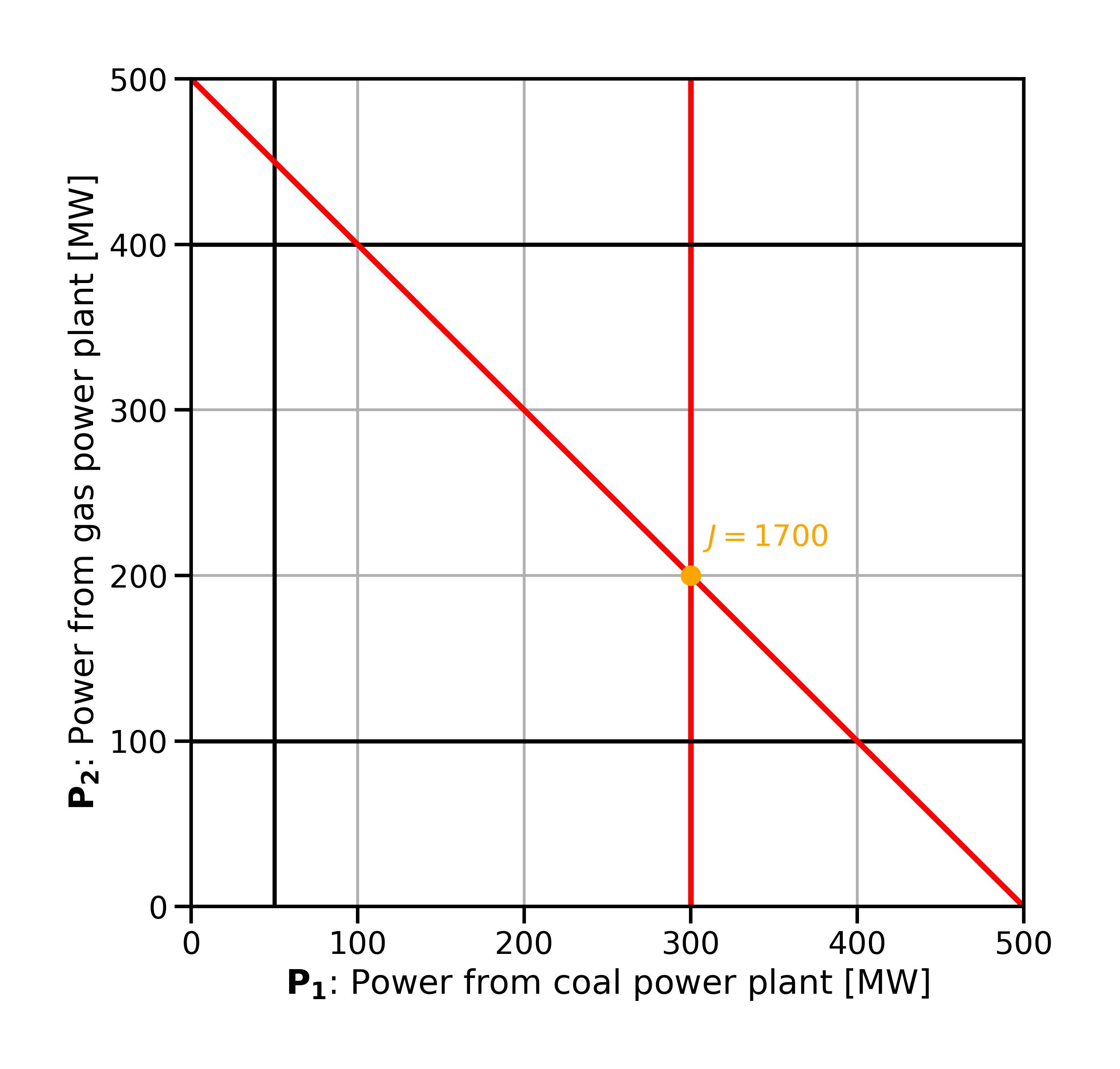
Fig. 2.9 Active constraints (highlighted red) in the economic dispatch problem.

More formally, if we have a constraint \(g(x) \leq 0\) then this constraint is active (binding) at \(x\) if \(g(x) = 0\) and inactive (non-binding) if \(g(x) \lt 0\). The active set is the set of constraints that are active at the current point.

2.7. Solving LP problems algorithmically

So far we looked at a simple case with only two dimensions, which allows us to represent the problem graphically. In addition, our feasible region is so simple that we had only two extreme points to examine for the optimal objective function value. Let’s modify the demand constraint from an equality to an inequality constraint:

(2.7)\[\begin{equation} \label{eq:ed_balance_modified} P_1 + P_2 \leq 500 \end{equation}\]

This does not necessarily make a lot of real-world sense - in our problem formulation we are minimising cost and so we would expect that electricity generation is as small as possible if there is no equality constraint that forces the model to deliver a certain demand. And indeed the new optimum is \(J = 550\) (Fig. 2.10).

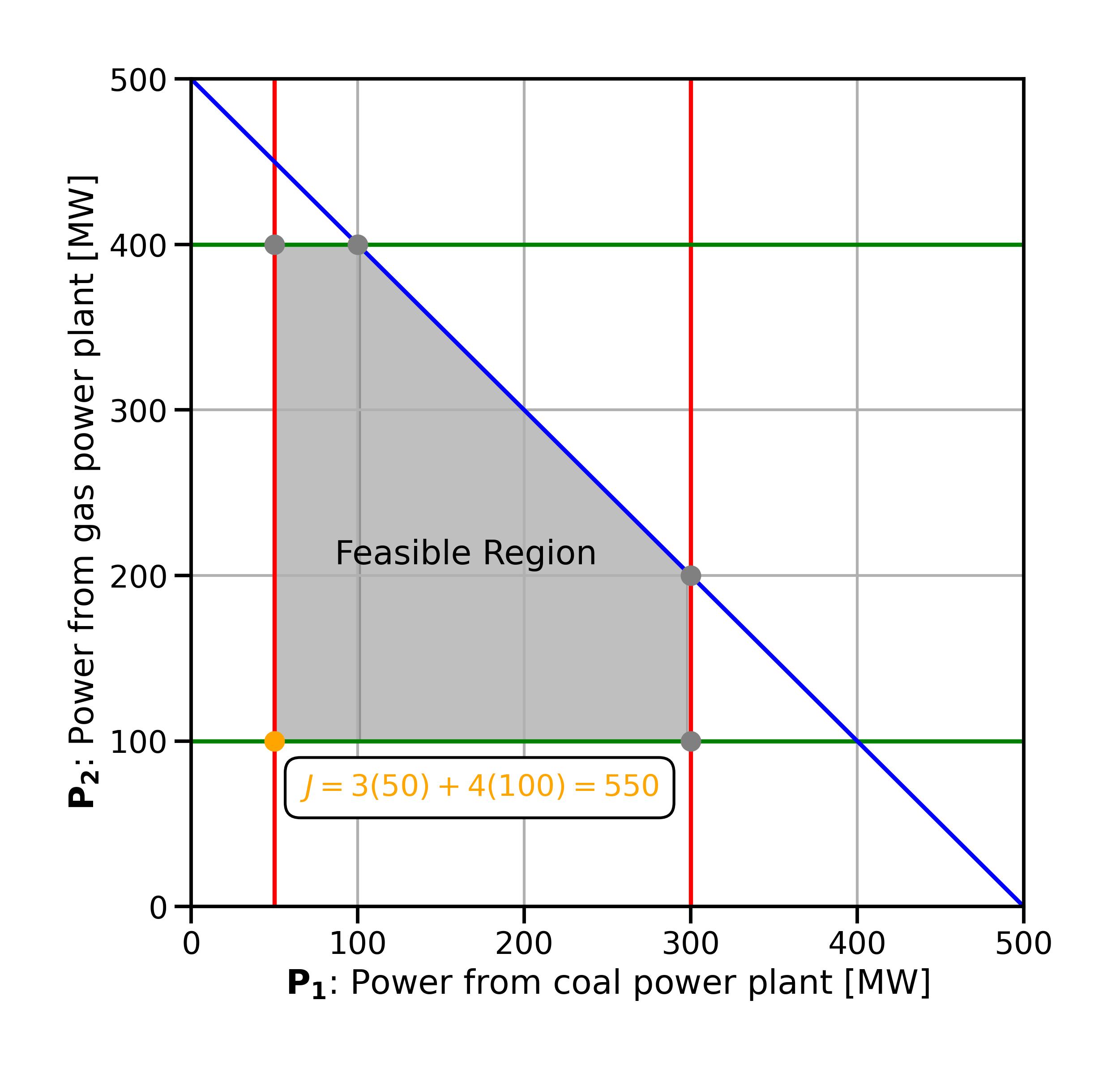
Fig. 2.10 Optimal solution with demand constraint changed from an equality to an inequality constraint.

Again, for this two-dimensional problem, the contour lines can help to give an intuition about why this is the optimal solution: we go downhill along the contour lines within the feasible region until we are stuck in the “lowest” corner and cannot go any further (Fig. 2.11).

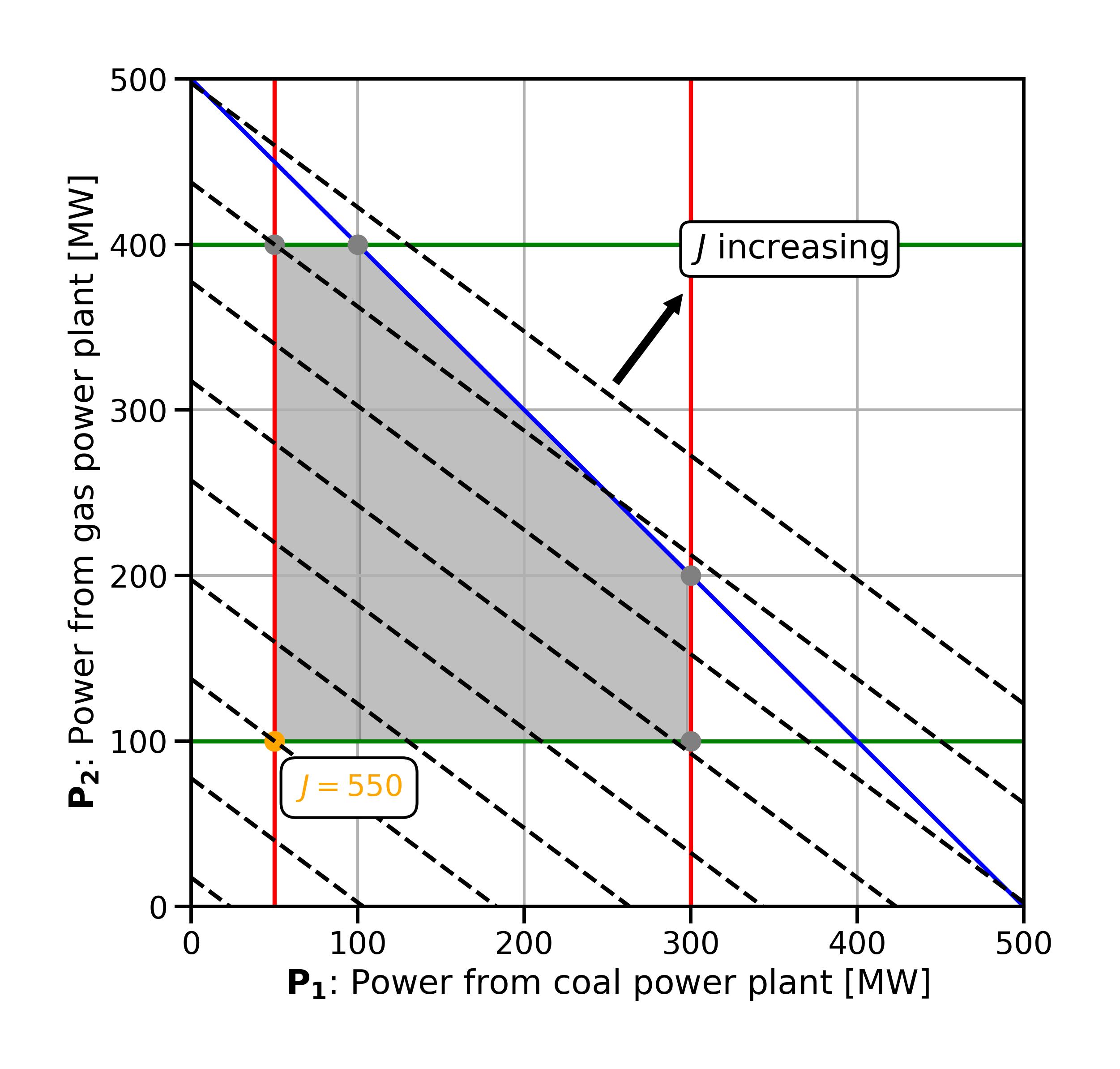
Fig. 2.11 Contour lines in the modified problem.

But what about problems with three dimensions or more? For example, if we have four power plants, we have four decision variables, so we have a four-dimensional problem which already is impossible to draw or solve graphically. However, even in \(n\) dimensions, the optimal solution would still be at an \(n\)-dimensional extreme point. And moving within the feasible space in the direction of increasing or decreasing objective function value would lead to that optimal solution.

In principle, even for very large problems, we could calculate the objective function value at all extreme points. But that might take a very long time. Luckily, very powerful algorithms exist that can solve even very large problems. The simplex method is one such algorithm. It was developed by George Dantzig in the 1940s and today is still the most popular algorithm used to solve linear optimisation problems. It begins by identifying an initial extreme point and then examines neighbouring extreme points. The algorithm calculates the objective function’s value for each neighbouring point and moves to the one with the best value. The process continues until no better value is found, at which point the algorithm stops: the current extreme point is the optimal solution. This method skips many points, checking only those that are likely to improve the result. Therefore it is computationally feasible even for large problems.

Fig. 2.12 illustrates this for a three-dimensional problem (with three decision variables), where we can still illustrate the process graphically. We will not look at the specifics of the simplex algorithm, but the intuitive understanding we gained above by using contour lines in two-dimensional problems gives us a sense of what the simplex algorithm does.

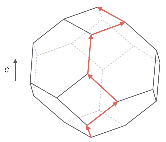
Fig. 2.12 A three-dimensional linear optimisation problem and the Simplex algorithm’s path towards its optimal solution. The objective is to maximise the value of the objective function c. Adapted from Figure 9.16 in Moore and Mertens [2011].

Convex optimisation

Linear optimisation problems are a subset of the general class of “convex optimisation” problems. Convex optimisation means that we are dealing with convex functions over convex regions and makes the above approaches to finding a solution possible.

2.8. General formulation of an LP problem

So far, we have discussed a specific example - a simple economic dispatch problem of two power plants. In this simple case, we have two variables, so it is a two-dimensional problem that we can plot in two-dimensional space and thus solve graphically. More generally, an optimisation problem can be arbitrarily large and have many dozens, thousands, or even millions of variables. A more general formulation of an LP problem follows with \(n\) variables is as follows.

Our 0 parameters are \((a_{11}, a_{12}, \ldots, a_{ij})\) and the 1 variables are \((x_1, x_2, x_3, \ldots, x_n)\).

The 2 objective function is:

(2.8)\[\begin{equation} f(x) = c_1x_1 + c_2x_2 + c_3x_3 + \ldots + c_nx_n \end{equation}\]

\(c_1 \ldots c_n\) are the objective function coefficients.

We optimise (maximise or minimise) the objective function subject to a number of 3 linear inequality constraints of the form:

\[a_{11}x_1 + a_{12}x_2 + a_{13}x_3 + \ldots + a_{1n}x_n \leq b_1\]

\[a_{21}x_1 + a_{22}x_2 + a_{23}x_3 + \ldots + a_{2n}x_n \leq b_2\]

\[\ldots\]

\[a_{m1}x_1 + a_{m2}x_2 + a_{m3}x_3 + \ldots + a_{mn}x_n \leq b_m\]

The largest or smallest value of the objective function is called the optimal value, and a collection of values \((x_1^*, x_2^*, x_3^*, \ldots, x_n^*)\) that gives the optimal value is called an optimal solution.

2.8.1. Standard form

When formulating or dealing with problems that are small enough to write down, it is often easier to first transform them into a standard form. We can write a standard form problem as an objective function \(f\) together with inequality constraint functions \(g\) and equality constraint functions \(h\):

(2.9)\[\begin{align} \text{Min.} \; & f(x) \\ \text{s.t.} \; & g_i(x) \leq 0, \quad i = 1, \ldots, n \\ & h_j(x) = 0, \quad j = 1, \ldots, n \end{align}\]

There is no universally agreed upon standard form. You will see slightly different formulations described as standard form elsewhere, for example a maximisation rather than a minimisation or different constraint notations.

To convert a problem into our chosen standard form, we can turn \(\geq\) inequality constraints into the form of \(\leq\) constraints through multiplying by \(-1\). Similarly, multiplying the objective function by \(-1\) changes a minimisation into a maximisation problem. So minimising \(f(x)\) is equivalent to maximising \(-f(x)\).

To convert a problem like the one in Section 2.8 into standard form we also move any constant coefficients onto the left-hand side of the constraints. Putting all of this together, we might turn a constraint like:

(2.10)\[\begin{equation} 2x_1 + 4x_2 \geq 10 \end{equation}\]

Into the equivalent:

(2.11)\[\begin{equation} -2x_1 - 4x_2 + 10 \leq 0 \end{equation}\]

2.9. Further reading

The following chapters in Hillier and Lieberman [2021] are particularly relevant:

• “Introduction to Linear Programming” for more mathematical background and additional examples

• If you want to understand how the simplex algorithm works, “Solving Linear Programming Problems: The Simplex Method” and “The Theory of the Simplex Method”

2.10. References

[HL21]

Frederick S. Hillier and Gerald J. Lieberman. Introduction to Operations Research. McGraw-Hill Education, New York, NY, 11th edition, 2021. ISBN 9781259872990.

[MM11]

Cristopher Moore and Stephan Mertens. The Nature of Computation. Oxford University Press, Oxford, UK, August 2011. ISBN 9780199233212.